1 Preface
The Worker process is in its function independent of the Chief process. It is designed to continuously process the video, calculate the camera pose and forward this information to the Chief process. All of this is done in real time. For Pixotope Vision, Marker and GhosTrack, the video of a sensor camera is used in the Worker, for Pixotope Fly the video of an aerial camera.
Setting up the Worker consists of two parts:
-
The 3D-scanning of the environment, solely based on the video.
-
Setting the coordinate systems position, orientation and scale
1.1 Working Principle
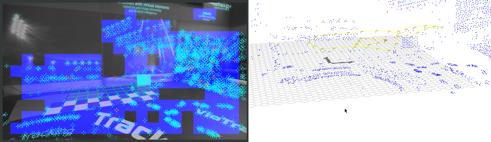
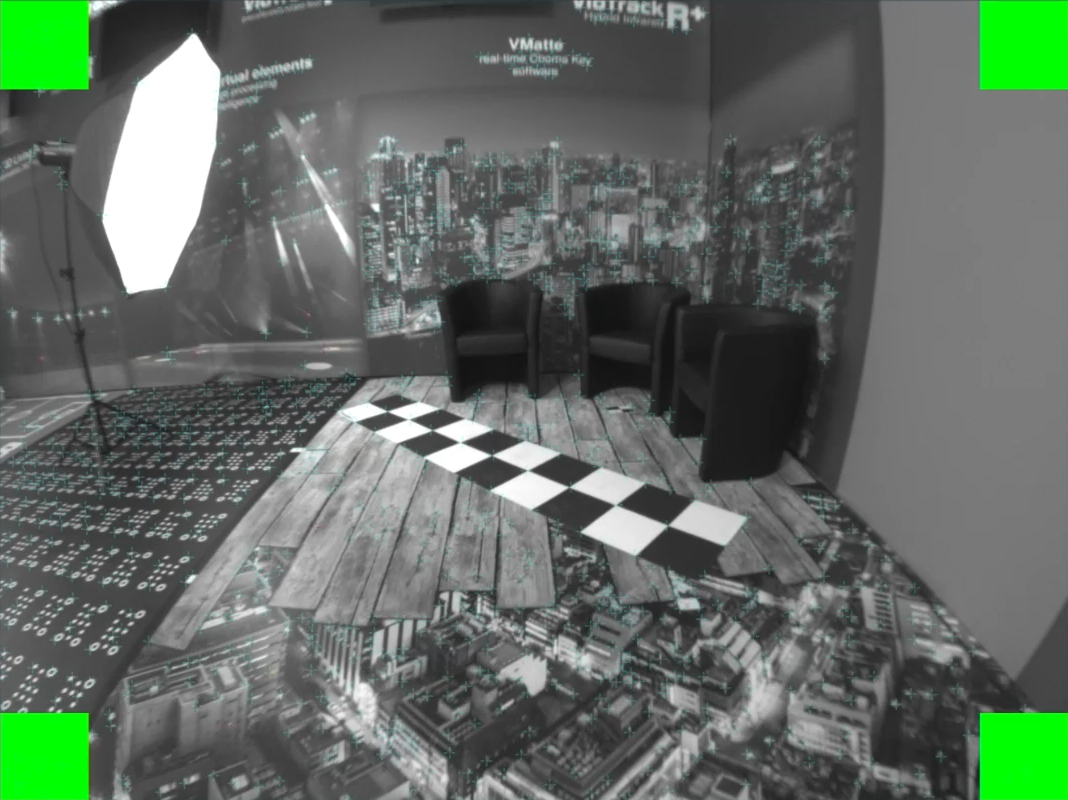
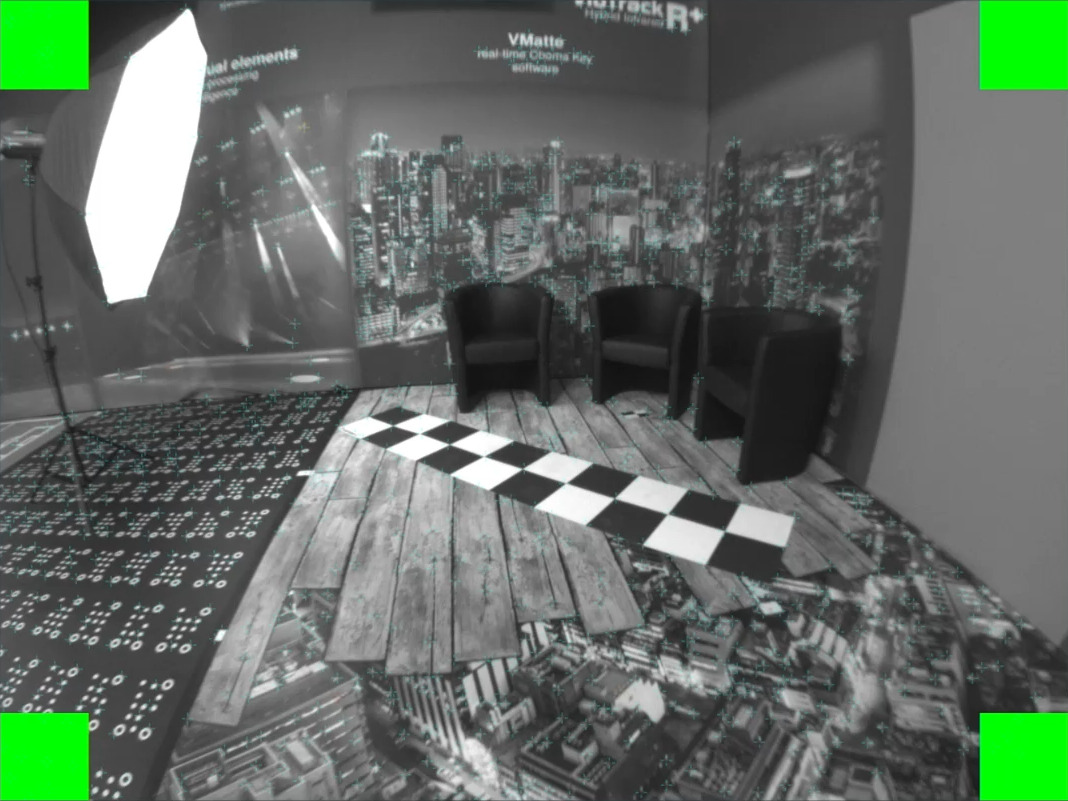
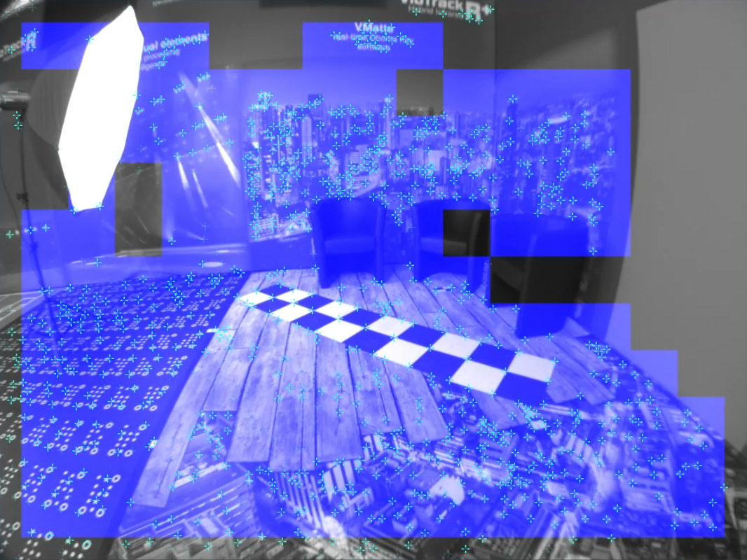
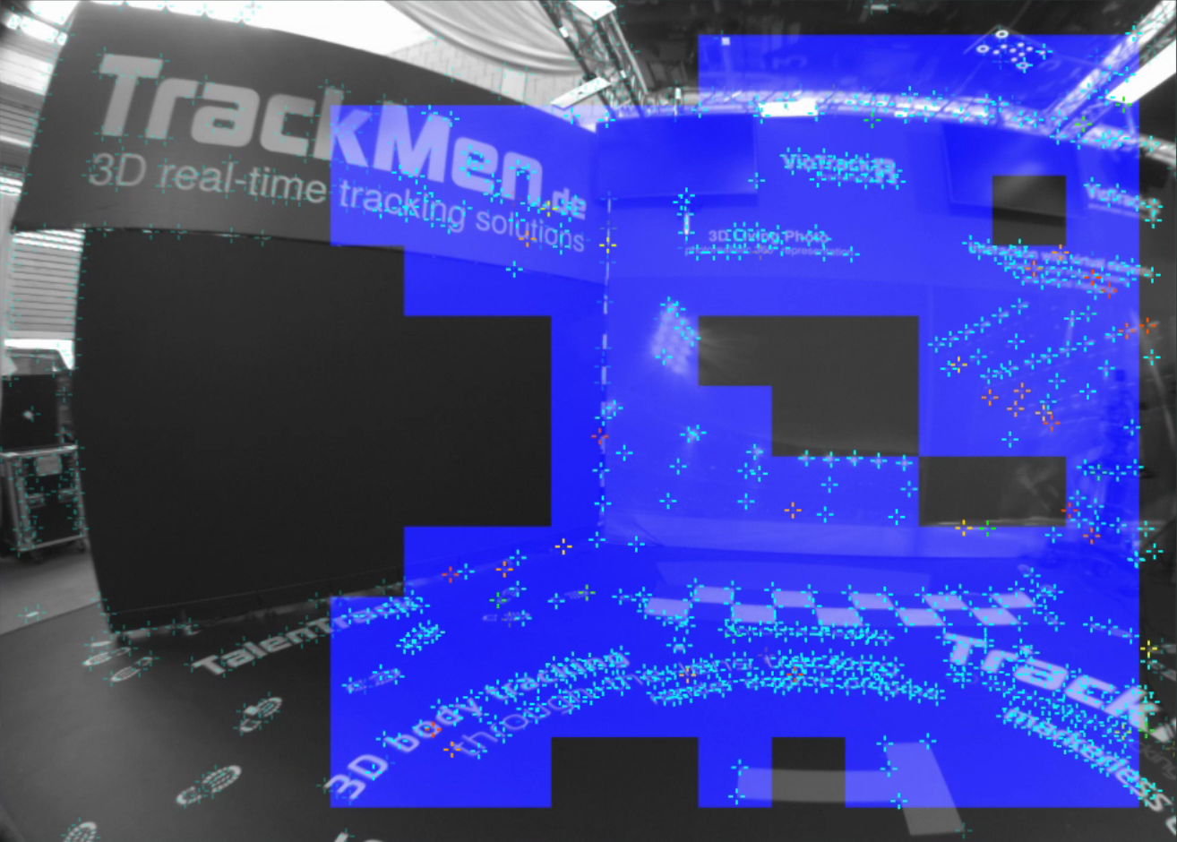
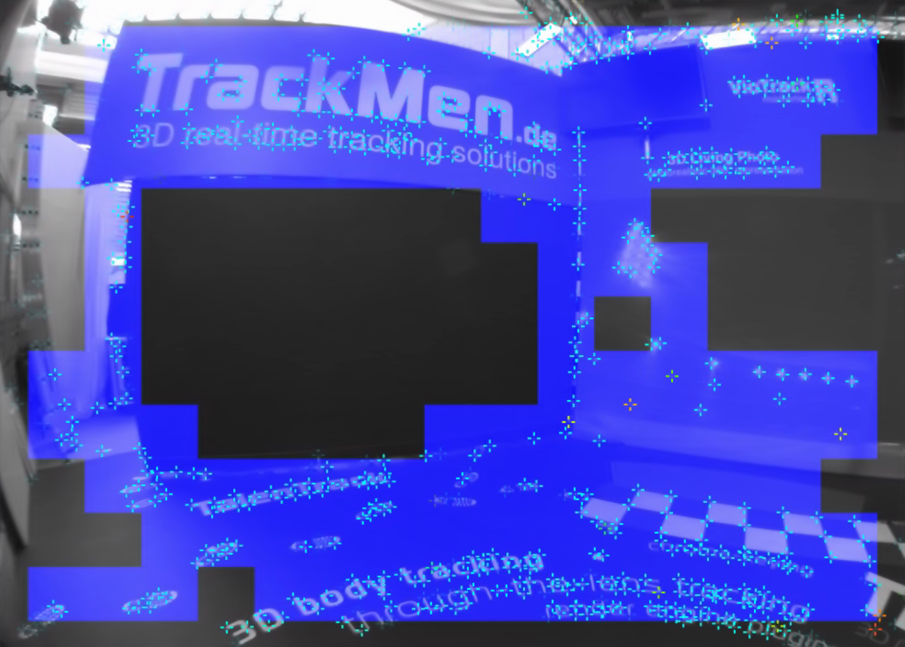
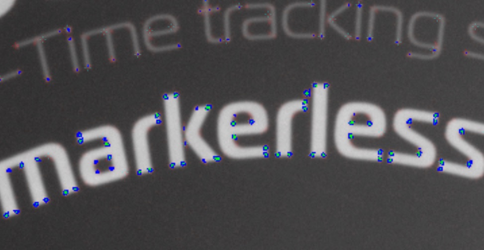
When scanning the environment, a 3D point cloud will be created based on well visible points in the video. These points are called feature points, indicated by small blue crosses in the video. The orientation of the coordinate system and also the scale are defined afterwards. This data is saved as a Reconstruction. When a reconstruction is loaded, recognized areas are indicated by blue squares in the video. Blue squares in the Worker video indicate that tracking data is generated and forwarded to the Chief.
If the positions of feature points change because objects have been moved or illuminated differently, the program will disregards those points for tracking. If the changes become increasingly excessive the Reconstruction can easily be updated. Also adding new areas to the Reconstruction is an easy and quick process. The program allows to switch between different Reconstructions, for example when moving the camera into another studio or changing to another lighting.
1.2 Sensor Unit
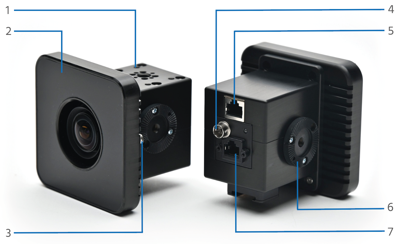
A sensor unit consists of a sensor camera providing the video for the Worker, a motion sensor (IMU) for tracking data enhancement and an optional infrared ring-light for using reflective markers. The casing offers multiple mounting options.
This manual focuses on the use of a sensor unit. See the Pixotope Fly manual for the use of an aerial camera as a Worker video input.
-
Screw holes for the standard mounting bracket
-
Optional infrared ring light
-
Power connector for the infrared ring light
-
Power connector for the sensor camera
-
IMU connector RJ45
-
ARRI rosette mount
-
Sensor camera network connector RJ45
2 Requirements
2.1 Video input
The sensor camera is a network camera, connected via a Link-Local connection. This means there must be a direct and exclusive connection between the sensor camera and the computers ethernet port.
The cable must be of high quality, shielded and capable to transmit at least 1 Gbit/s.
The computers' ethernet port that the sensor camera is connected to has to be selected in the ZeroConf network connection. See chapter 6.2.1 of the OS manual for more information about this.
For sensor camera network requirements go here.
2.2 Lens file
For creating a Reconstruction the final fixed lens calibration file (the one that will be used during production) has to be selected in the Camera tab.
See the respective manual on how to create a fixed lens calibration file.
2.3 Tracking area
Before creating a Reconstruction, the tracking area, meaning the area that is providing feature points, has to be prepared.
-
Make sure that the area to be reconstructed is as similar as possible to how it will be during on-air use of the tracking:
-
no significant visual changes for the sensor camera
-
not more than necessary markers are occluded
-
the lighting is similar and as close as possible to show lighting
-
-
Make sure that reliable tracking is always possible:
-
there are always enough feature points in the cameras view in every camera position and orientation that will be used on-air
-
the feature points are spread out in 3D space of the tracking area as well as in the video
-
the cameras view onto the feature points is not obstructed in any position or orientation
-
-
3 points for establishing the coordinate system are marked and well visible in the tracking area during the process of creating the reconstruction.
3 Setup
3.1 Worker Video
-
Start the Worker from the Tracking menu in the task bar
-
Open the Settings and go to the Camera tab
-
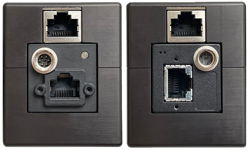
Select Spinnaker or Vimba as the Interface type depending on the model of the sensor camera. Vimba models have an ethernet port that is 90 degrees rotated to the side
-
Click on Change image source. The video should now appear in the main Worker window
-
Choose the fixed lens Calibration file for the sensor camera
Two things can interrupt the connection to the sensor camera. In both cases the network connection has to be actively reestablished by the software once the problem has been resolved:
-
The sensor camera not receiving power input. It takes approximately 25 seconds after powering it on to fully boot. Check if the sensor camera is powered and is fully booted and click Restart Image source in the Camera tab
-
The network connection being disconnected. This may be a broken or bad cable too. Check the network connection and click Restart Image source in the Camera tab
3.1.1 Automatic Restart
The latest software version can reestablish the connection automatically when the signal is lost.
-
Open the settings and go to the Camera tab.
-
Activate Show expert settings
-
Change Automatic restart delay to the desired value of seconds after which the software should try to restart the image source
In older software versions the connection can be reestablished manually by clicking on Restart Image source in the Camera tab or by restarting the Worker software.
3.2 Camera Tab
For a good feature point detection, a generally bright image of the sensor camera should be aimed for. Change the sensor camera settings while it is seeing the environment that will be reconstructed under show lighting conditions. This allows optimizing the feature point detection.
Open the Settings and go to the Camera tab:
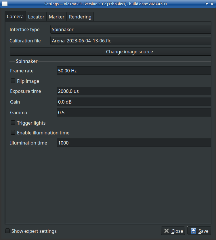
3.2.1 Frame rate
The frame rate of the sensor camera must be equal to or higher than the video frame rate of the tracked film camera during production. This ensures having correct tracking data for every frame of the film camera.
3.2.2 Exposure time
Increasing the Exposure time increases the brightness of the image, improving the feature point detection. At the same time this increases motion blur in the video during movements. An exposure time that is too long can cause tracking drop outs during very fast movements. Avoid an Exposure time over 4000μs. 2000μs is the default value, viable for most use cases.
3.2.3 Gain
Gain can be use to increase the brightness of the video, also improving the feature point detection. The increased image noise can introduce jitter to feature points. Keep the Gain rather low and avoid values higher than 15dB.
3.2.4 Gamma
The Gamma should in most cases be 0.5, allowing the system to see more details in darker parts of the image. The lower contrast is a good tradeoff for the increased amount of details.
3.2.5 Infrared light
Trigger lights, when active, turns the Infrared LEDs in the sensor unit on. This is obligatory in case infrared markers in the form of reflective material is used. The Illumination time determines the intensity of the LEDs. Activate Enable illumination time and adjust this value for an ideal visibility of the corners of the markers while maintaining a high contrast.
3.3 Locator Tab
The Distance factor determines how many keyframes are taken automatically when creating or extending a Reconstruction. It can vary between 0.05 and 0.25. For the beginning a default value should be set. In case of problems occurring or a sub-optimal performance, the Distance factor can be modified and the Reconstruction process started anew.
Open the Settings and navigate to the Locator tab. Change the Distance factor to match the use case. Start with default values:
0.10 for small studios/environments
0.15 for large studios/environments
Read chapter 6.3 for more information about the Distance factor.
3.4 Marker Tab
The Marker Tab is only used for Automatic Initialization setups utilizing the coded absolute markers.
3.5 Rendering Tab
Make sure that Draw grid is active. The grid in the Worker video is an essential method to determine the quality of the tracking.
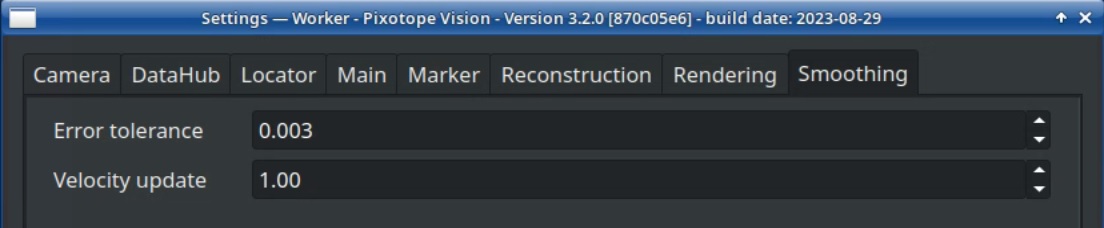
3.6 Smoothing
Open the Settings, Activate show Expert Settings and navigate to the Smoothing tab. When using a sensor unit, set Error tolerance to 0.003 and Velocity update to 1.0. Also see chapter 6.7 about Smoothing.
4 Operation
Creating a new Reconstruction is always a two-step process. First the area has to be scanned to create the 3D point cloud. Then the origin, the orientation and the scale of the coordinate system have to be defined. The software calculates the 3D position of the sensor camera in relation to that coordinate system.
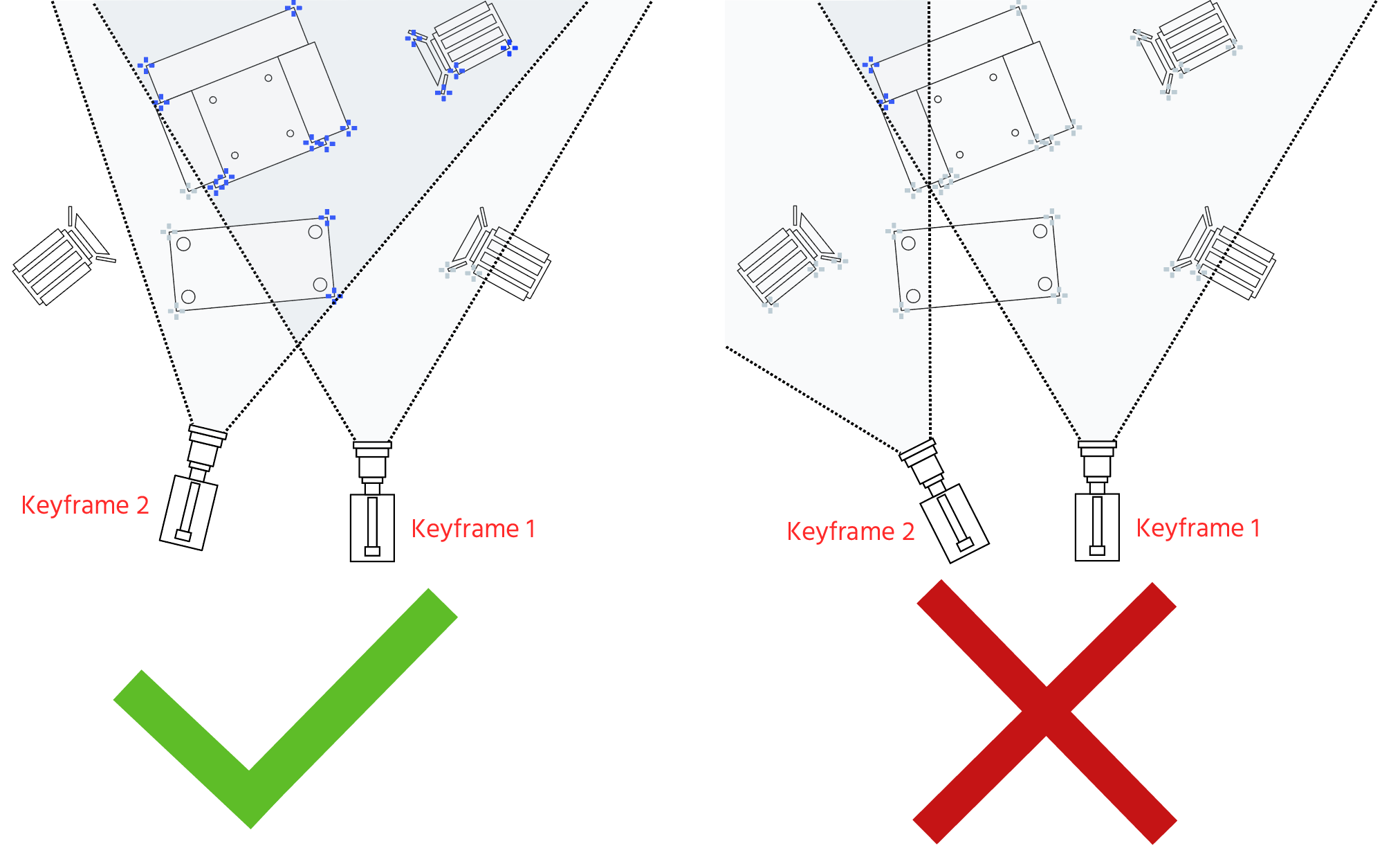
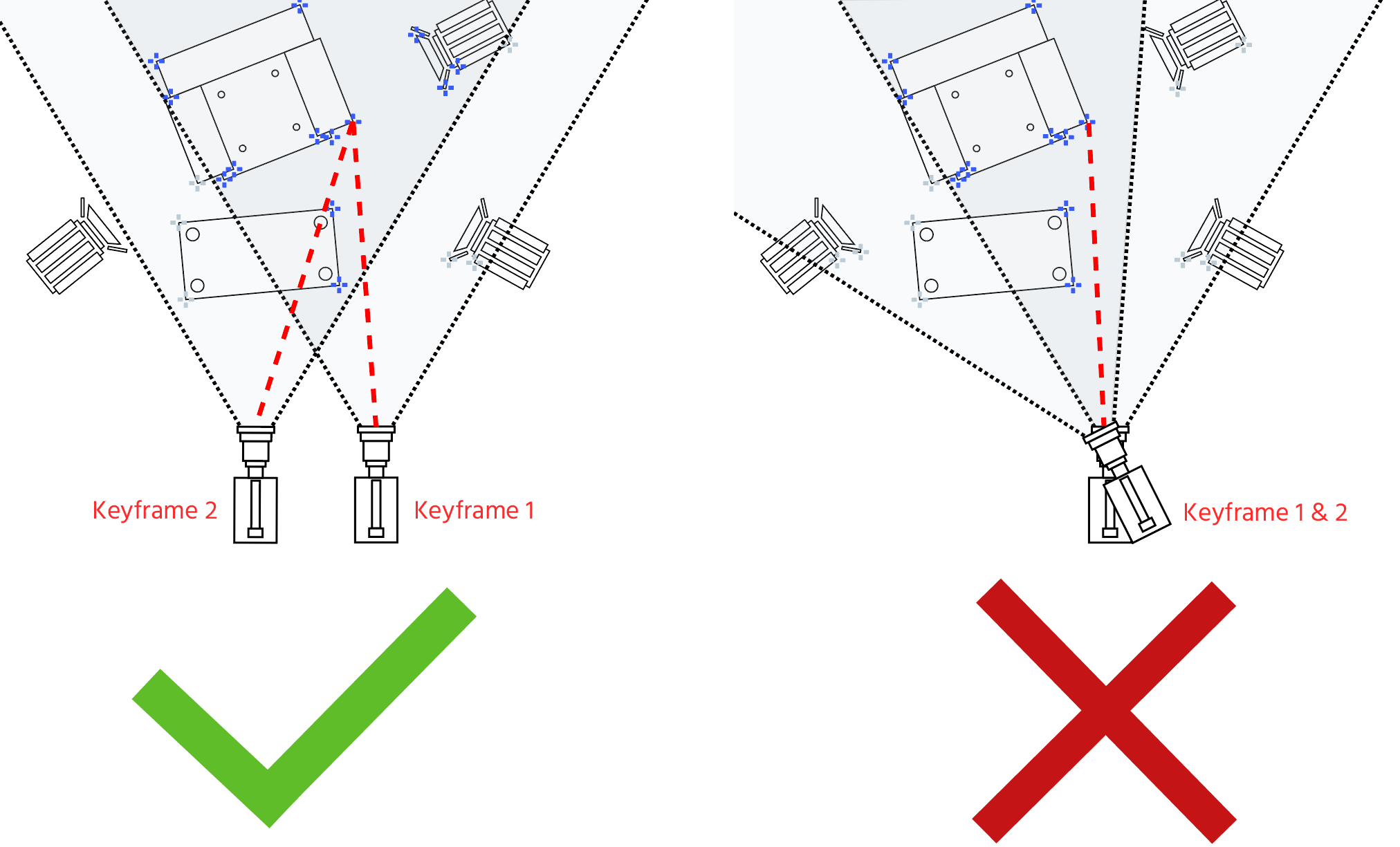
Pixotope Tracking is a monoscopic system, which means that for gaining 3D information it needs to see each point from at least two different camera positions. The calculation of each points' 3D position is done by the means of triangulation. The consequence is that for scanning an environment the camera has to move in 3D space during the process. Panning or tilting, when not combined with movement, is counterproductive.
To start building a Reconstruction two keyframes are set manually from positions that are approximately half a meter apart. This creates the first 3D information. After this initialization, Allow Extension activates automatically and the camera just needs to be moved. The program notices changes in perspective and adds keyframes automatically, extending the point cloud.
Please also refer to the Initialization video tutorial, the ceiling reconstruction video and the Pixotope Fly video for a visual representation of the processes in this page.
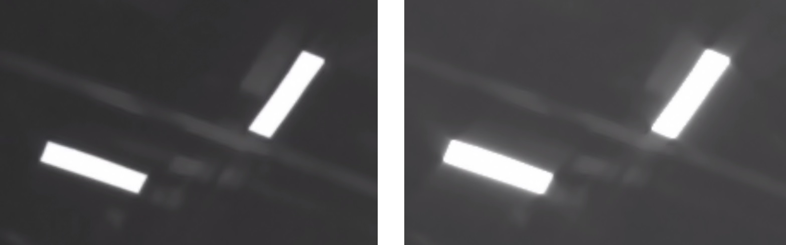
4.1 “Learning” the environment
-
Start the Worker
-
Press Reset to remove any already loaded Reconstruction
-
Have the camera see the area you want to reconstruct and if needed adjust the camera settings
-
Press Set Keyframe:
-
After taking the first keyframe, move the camera approx. half a meter to one side. Also pan slightly. It is important that the camera, while moving, keeps seeing mostly the same objects it has seen when taking the first sample; in the end of the movement from a different perspective and position
-
Press Set Keyframe again
-
You should see blue tiles appear in the video. This represents the areas where the system recognizes 3D information
-
Feature points that get lost between taking the first and second keyframe will not be reconstructed. It is therefore important between the first two keyframes:
-
not to obstruct the cameras view of the feature points
-
not to pan or tilt in a way that too many feature points leave the cameras frame
-
Move the sensor unit around the area so the system can capture feature points efficiently
-
Check Allow extension if it is not already checked. This allows the automatic capturing of frames after initialization. Any loss of the tracking (no blue squares in the image) will deactivate Allow Extension
-
The Distance factor determines how many keyframes the program takes automatically. For more keyframes decrease the value, for less keyframes increase it
-
You can click Add Sample at any time to manually add samples to your Reconstruction
-
Avoid fast movements. This will introduce motion blur in the sample and provide bad data for the Reconstruction
-
When taking keyframes always combine camera rotation with movement. Panning or tilting alone does not provide proper 3D information of the environment.
The more perspectives you capture from a feature point, the more precise its 3D information becomes.
-
To add new areas, always have already reconstructed feature points in view. Only then can newly seen feature points be added to the point cloud.
-
When you are happy with the Reconstruction, uncheck Allow extension
-
You can click on Save Reconstruction to save the point cloud, but this will save the Reconstruction without a correct transformation. The correct transformation will be set in the next chapter
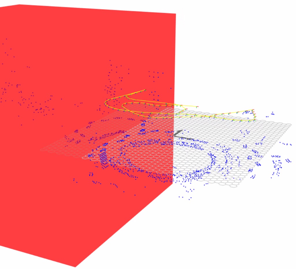
You can click Enable 3D View to see a visual representation of the point cloud.
4.2 Setting Transformation
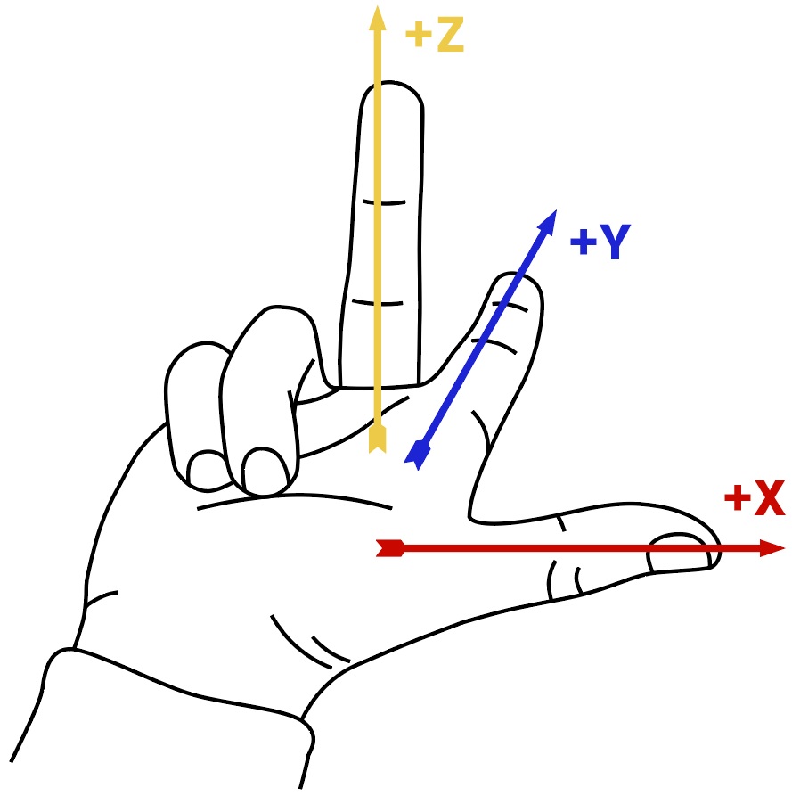
Pixotope Tracking uses a “right hand coordinate system”. To visualize the interpretation of the axes you can use your right hand as shown in illustration 10. X and Y will define the floor (zero) plane and Z+ will point upwards.
A coordinate system is defined by three points on a plane. In most cases that should be the floor.
4.2.1 Set Coordinates
The Set Coordinates sub menu allows to define the origin and orientation of the coordinate system within keyframes as well as the scale. Placing stickers or the Pixotope roll up checker board can help providing feature points where they are needed.
Choose three points inside the tracking area for defining the orientation and the scale. These 3 points must be on the same plane. This will create the zero plane, so ideally they should be on the floor. The three points have to be reconstructed from different perspectives and each one of them must be included in at least two keyframes. It does not matter which keyframes they are in. Before refining the coordinates make sure each of the three points is well visible in at least two keyframes.
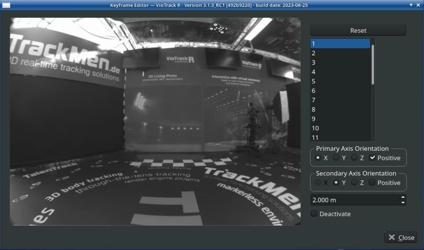
Refine Coordinates overwrites all settings set in the right side of the Worker window as shown in Illustration 12.
-
Open the Settings menu and navigate to the Locator Tab
-
Click Refine Coordinates. This opens the Keyframe Editor window
-
On the right side you can see a list of all keyframes that were taken
-
Select a keyframe where one or multiple points are well visible
-
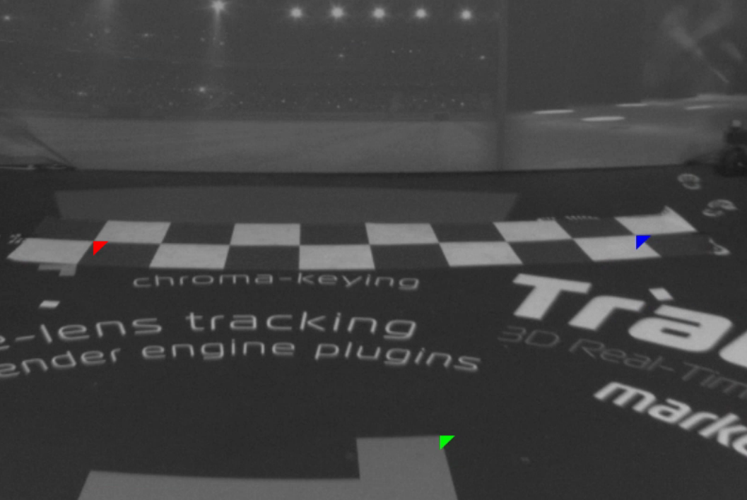
Left-click on them in the following manner:
First Point:
Origin
Second Point:
Primary axis, starting from the origin
Third Point:
Direction of Secondary axis. The Secondary axis starts from the origin and is always 90° to the Primary axis
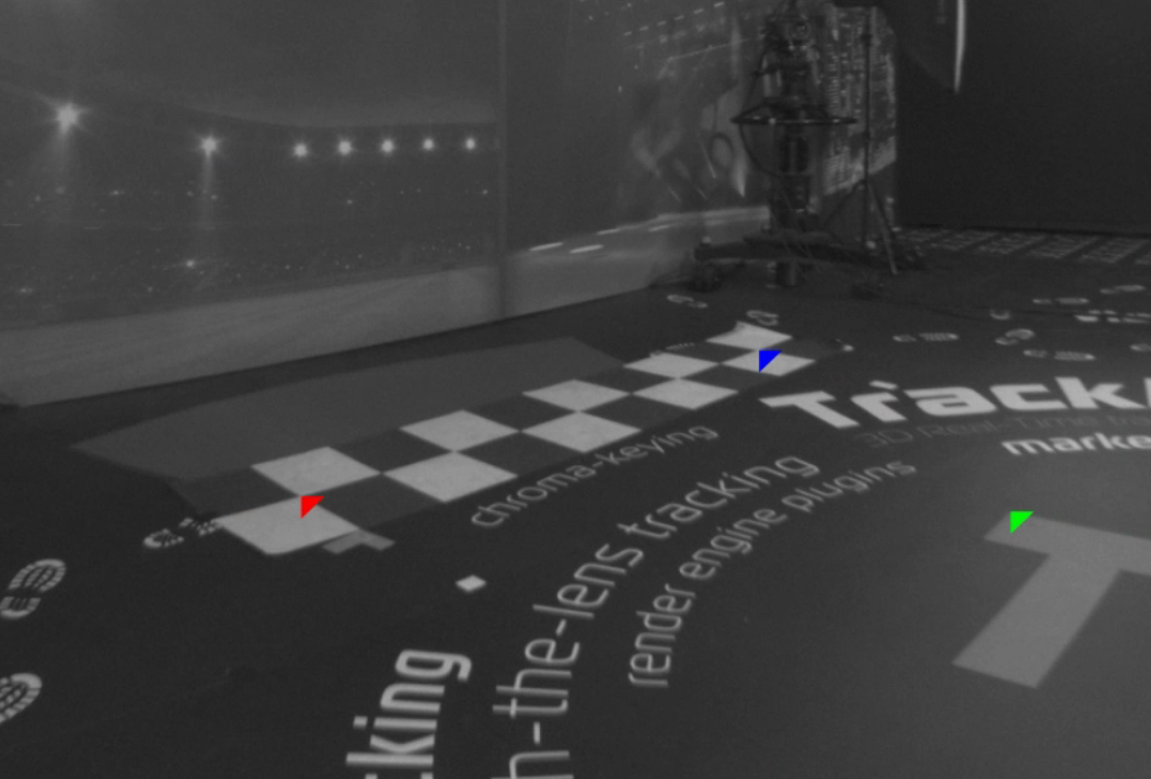
Use the mouse wheel to zoom into the keyframes in order to have the triangle point to the exact location with high precision.
-
Do the same thing in multiple keyframes. These keyframes must have a significant difference in perspective to one another. The position of each point has to be defined in at least two different keyframes
The triangles can also be dragged and dropped. To remove a point, right-click on it.
Increase the precision of the tracking:
-
by refining the coordinates in more than two keyframes
-
by refining the coordinates in keyframes which are significantly different in camera position / perspective.
-
Choose points with both high contrast and a corner that is well visible. This enables you to click on the exact same point from different perspectives.
-
Define Primary Axis and Secondary Axis Orientation in the menu on the right side. The menu let’s you assign Primary and Secondary axis and their direction. The third axis is a consequence of the first two, being 90° to both of them. Keep the “right hand system” (Illustration 10) in mind while defining
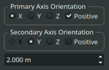
-
Define the scale by inserting the real world distance between the first two points (red and blue) in meters
-
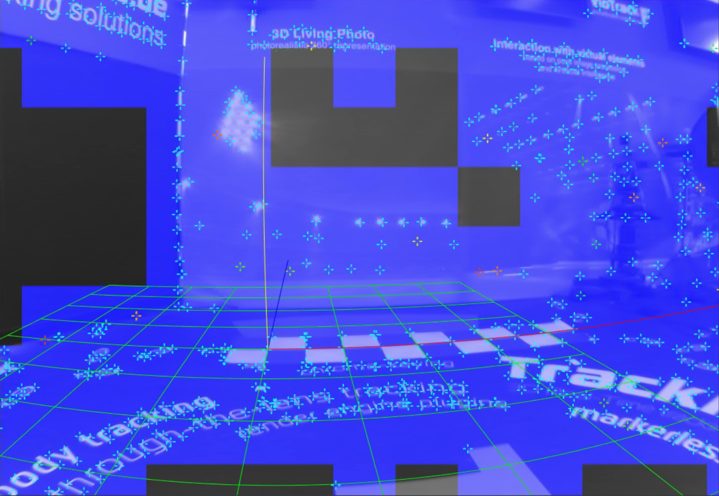
Close the Keyframe Editor and control the Worker video. A grid is displayed in it showing the applied transformation that was done using Refine Coordinates:
-
Red line: X-axis
-
Blue line: Y-axis
-
Yellow line: Z-axis
-
The default grid consists of 0.5m squares
-
The settings for the grid are in the Rendering tab in the Settings (see chapter 6.6)
-
If the grid sits correctly from all perspectives, click Save Reconstruction. This saves the point cloud together with the transformation. Every time you save a Reconstruction the system will create a new version of the Reconstruction. It will never overwrite an existing Reconstruction.
4.3 Handling Reconstructions
Reconstructions are saved in the /home/tracking/pxVision/ directory. Each one creates a new folder starting with “VioTrackR_Sequence…”, consisting of the keyframes and data files.
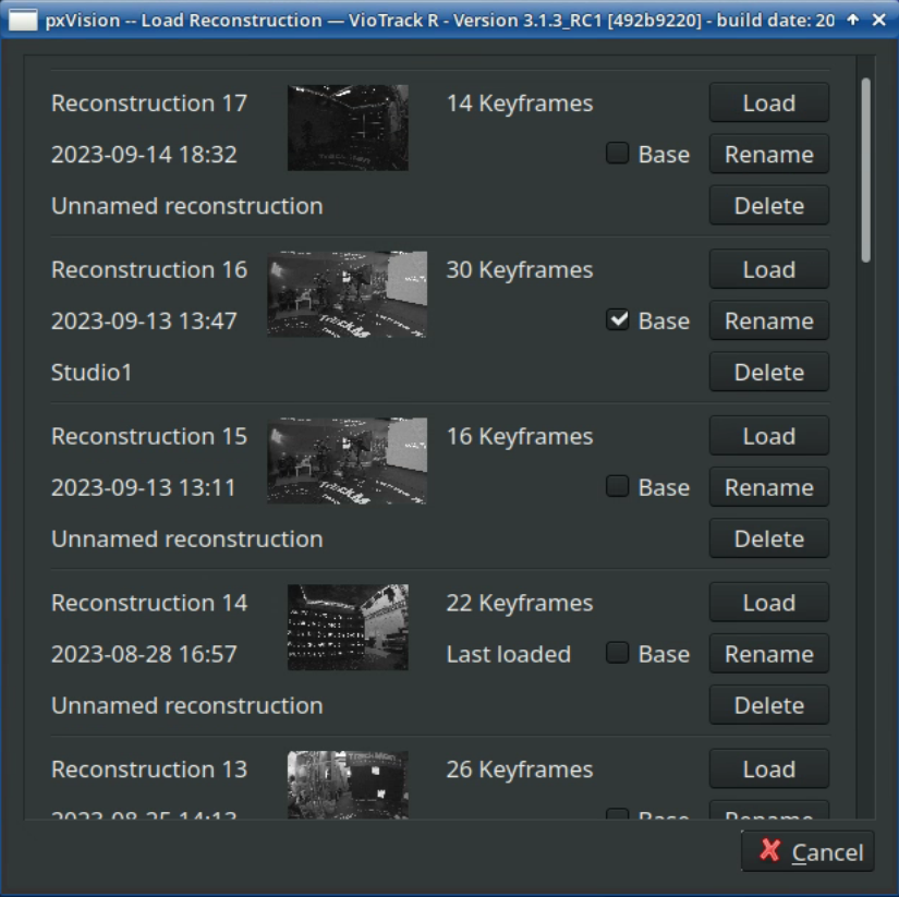
When clicking on Load Reconstruction in the Worker window a chronological list of all Reconstructions will open in a new window. Here the Reconstructions can be loaded, renamed and deleted.
By default the Worker will always load the most recent Reconstruction when the software is started. Only when you activate the Base checkbox from a Reconstruction, it will always load that one.
4.4 Extending an existing Reconstruction
If the position of feature points changes because the objects are moved or illuminated differently, they will no longer be available for tracking. If changes become too many, the recognition and recovery when starting the tracking can take longer or even fail. In that case new keyframes can be taken to update the point cloud.
Also when many new feature points have been added to the tracking area, new keyframes should be taken to add them to the point cloud.
Keep in mind that every new or changed feature point has to be included in at least two new keyframes, which are taken from different perspectives.
-
Point the camera to see the areas you want to update
-
Add a keyframe
-
Move the camera to see the points from a different perspective without losing the view of them
-
Add another keyframe
-
Repeat until at least two keyframes have been taken of every new feature point
If many keyframes have been added, it should be checked whether the performance is still unproblematic (see chapter 5).
Alternatively Allow Extension can be turned on and the camera moved. This way the software will take keyframes automatically if it notices significant changes to the old keyframes. The amount of change it takes for the software to add a keyframe is determined by the Distance factor. The Distance factor might need to be lowered in order to take enough keyframes or increased in order to avoid too many keyframes being taken and running into performance problems.
5 Performance Diagnostics
The software is obliged to provide correct tracking data for every frame of the video in real time. In order to do so it needs to process all information gathered during the creation of the Reconstruction for every single frame. That includes all feature points and keyframes. Increasing the amount of feature points, the amount of keyframes or the amount of details visible in the video increases the time the software needs to calculate the tracking data. If the processing load for a frame is too high, the calculations might not be finished in time, resulting in a dropped frame. This means that a Reconstruction cannot be infinitely large. The limit is the real time capability set by the computers hardware.
The performance is directly related to the hardware specifications of the computer, especially the graphics card. Check the System Requirements for further information about the necessary hardware.
For controlling the performance of the Worker, it is possible to display a Performance Bar. To bring this additional tool up, enable it on the right side.
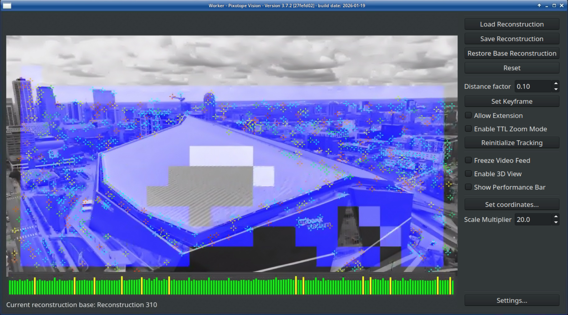
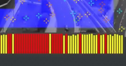
The colors of the bars show how close the calculation time for this frame is to the duration of the frame. When the calculations for a frame exceed the duration of a single frame, the bar of this frame does not show. The goal should be to have mostly green bars and no gaps. However, yellow bars are unproblematic and also single red bars do not result in a dropped frame.
The following settings can be adjusted to reduce the processing load:
-
Distance factor: Increasing the Distance factor reduces the amount of keyframes being taken with Allow extension active.
-
Minimum distance: Increasing the Minimum distance results in less feature points being detected in the video. Find more Information about the Minimum distance in chapter 6.3.
-
Score threshold: Increasing the Score threshold reduces the amount of feature points being added to the point cloud. Find more Information about the Score threshold in chapter 6.3.
The settings above take effect while creating or extending a Reconstruction. That means the Reconstruction has to be redone when choosing to use different values!
Repetitive patterns of drop outs in the delay chart can be caused by a faulty video input (Pixotope Fly), bad network connection or an active remote connection. These factors have to be eliminated before a final evaluation of the tracking performance is possible.

6 Expert Settings
Worker settings, which are not needed to be changed in most setups or are only meant for debugging and can be exposed by activating Show expert settings.
6.1 Camera Tab
Automatic restart delay
Determines the time after which the system tries to reestablish the connection to the sensor camera when the connection was interrupted.
Calibration directory
The directory for the fixed lens calibration files selectable in the Worker.
Device serial
When a sensor cameras devise serial is entered, the software automatically connects to this camera at start. Leave empty when using one sensor camera.
Flip image
Turns the video image by 180 degrees. This is useful in case the sensor unit has to be mounted upside down. Flip image should only be set to active, when the Flip image setting was active while creating the FLC and also while calibrating the offset.
Auto Gain
When active, the software automatically changes the Gain should the brightness of the environment change. Activating this should always be avoided. It makes the image brightness uncontrollable and thus the feature point detection unreliable.
Trigger delay / mode
This setting is only needed for GhosTrack applications.
6.2 Datahub Tab
URL
For XR setups that utilize Pixotope’s Digital Twin feature, enter the IP address of the Pixotope Server machine.
6.3 Locator Tab
6.3.1 Feature Detection
The image processing algorithm is based on the detection of high contrast corners. Two threshold values divide this detection into three different qualities of recognizability. These are called Score Threshold and Secondary score threshold. That means that the software detects features in the video with different qualities, depending on how well these features are recognizable. When activating Draw detection score in the Rendering tab, these differences become visible at the features in the video.
The detection score is indicated by a color code:
-
Red: Not very well visible features below the Secondary score threshold are disregarded
-
Blue: Well visible features above the Secondary score threshold but below the Score threshold are taken into account for the calculations
-
Green: Very well visible features above the Score threshold are taken into account with a higher weighting
Creating a Reconstruction with higher threshold values will result in having less feature points because feature points which are not well detectable are disregarded. The processing time will be shorter as a consequence.
6.3.2 Keyframes
The Distance factor determines how many keyframes the software takes automatically when Allow extension is active. It is a factor and therefore not based on a distance value but on the change that is happening to the feature points in the video. Changes happen when moving the camera in 3D space.
With a small Distance factor, a small change in the video causes a new keyframe being taken, meaning a smaller movement of the camera. For a high Distance factor more change/movement is necessary to cause a new keyframe.
The amount of keyframes that can be taken and saved has a limit because the amount increases the processing time of the software. The computer hardware sets this limit for real time capability. However, also the Minimum distance and the Score threshold have an effect of the processing time. Read chapter 5 for information about performance diagnostics.
The Angle threshold determines the maximum camera rotation angle allowed between taking two keyframes.
6.3.3 Minimum distance
The Minimum distance values determine the distribution of feature points over the detectable features in the video. The lower the values are the closer feature points can be to one another.
Increasing the Minimum distance values reduces the amount of total feature points, resulting in a shorter processing time.

6.3.4 Masking
It is possible to create masks in the form of cuboid volumes inside the point cloud. All feature points that are located inside a mask volume will be disregarded and not recognized in the Worker video. The software will check for each feature point if it lies within one of the masks and if yes, exclude this feature point from the calculations.
Masking out areas with many feature points that will not be used during production or that have change significantly can reduce the processing time and therefore improve the performance of the system. Using too many masks can also decrease the performance.
-
For adjusting masks Enable 3D View needs to be checked in the Worker menu on the right side of the window
-
Open the Worker Settings, navigate to the Locator tab and activate Show expert settings
-
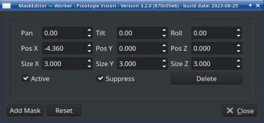
Activate Enable masking and click on the Masks… button
-
Click Add Mask to create a new mask
-
Activate Active and set Size X, Y and Z values to have the mask appear in the 3D view
-
Adjust Position, Size and if needed, Rotation to place the mask volume in the point cloud
-
To activate the masking function of the mask volume, activate Suppress
6.4 Main Tab
Logging
The Log level determines which messages from the Worker software are displayed in the System log. Keep in mind that the System log is not meant to be permanently observed but is an essential tool for error diagnostics.
Number of threads
Determines the multithreading on the CPU cores. The default value should be [number of physical cores (without SMT) - 2]. For example 4 for a CPU with 6 cores. This value can be changed depending on the hardware used. Older CPUs may yield better performance in single-threaded mode. In this case it can be beneficial to change the number of threads to 1. This should be verified using the delay chart.
6.5 Marker Tab
In case of an Automatic initialization setup, activate Automatic initialization and Use marker transformation; deactivate otherwise.
6.6 Rendering Tab
Draw detection score
Draws the detection score in the Worker video as described in chapter 6.3.1.
Grid
The Grid in the Worker video can be customized for the projects needs:
-
Open the Settings, navigate to the Rendering tab and activate Show Expert Settings
-
For the Primary and Secondary axes three settings can be adjusted:
-
Size refers to the distance between two lines on one axis
-
Tiles refers to the number of lines along one axis
-
Offset refers to the position of the origin in the number of lines
-
-
The Axes button selects which of the two axes define the grid’s orientation. This setting only affects how the grid is displayed in the Worker video and not the tracking data.
It makes sense to control the scale with the grid. Check the grid’s size values before.
Export Point data
Exports the positions of the feature points in a list of X, Y and Z values. The file being created is a text file.
6.7 Smoothing
The IMU provides redundant data on movement of the camera that is also used for stabilization in case of tracking data noise. So even if some shaking is noticeable in the grid of the Worker video, the virtual objects in the graphic engine should be still. In some cases, for example when having to work with subpar feature point coverage, it can still be necessary to apply a smoothing filter to the tracking data.
-
Error tolerance defines the amount of smoothing applied. When using a sensor unit it should not be higher than 0.005 or it may interfere with contradictory data from the IMU. The lower this value is, the less smoothing is applied
-
Velocity update filters the acceleration to counter erratic movements. This setting will affect the tracking delay, so be aware that the video delay will have to be adjusted when applying Velocity update. When using a sensor unit it should not be lower than 1
A smoothing filter can cause an effect that looks similar to a wrong delay. Having a good reconstruction and lens file in most cases allows not having to use a smoothing filter (Error tolerance of 0.000 and a Velocity update of 1.00). If the image noise in the form of shaking is still visible at the virtual objects, a minimal smoothing filter (Error tolerance of up to 0.005 and a Velocity update of 1.00) can be used.